Lotto game with Excel

Follow FullPress on Google

Add us to your preferred sources.

The tutorial “Lotto Game with Excel” organizes useful spreadsheets to keep track of lotto draws, delayed numbers, and case studies related to the lotto game.

• In our Excel file, we want to get a summary overview of the most important cases in the Lotto game. In this case, we cannot avoid a long data entry process, which we will only do the first time we open the file. Meanwhile, let’s establish that each spreadsheet corresponds to one wheel. So from the Insert menu, we choose Worksheet and repeat the operation until we have inserted “Sheet 10”, so that there is one for each wheel.

• From the Format menu, choose Sheet, then Rename. The sheet name appears selected and we can overwrite the name of the first wheel, alphabetically, Bari. Repeat the operation with the wheels of Cagliari, Florence, Genoa, Milan, Naples, Palermo, Rome, Turin, and Venice. The same operation can be done faster by right-clicking and choosing Rename from the appearing menu or by double-clicking on the sheet name and then overwriting it.

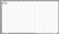
• Let’s try to automate data entry as much as possible. In the “Bari” worksheet, in the first row, we will mark the dates of the draws starting from cell B1. Select the first row and choose Cells from the Format menu. On the Number tab, choose the Date category and the type you like the most. On the Font tab, choose the Bold style. To enter the dates, just type the day and the first three letters of the month, for example “17 sett”. The spreadsheet will display the chosen date type, “17-Sep-03”.

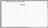
• In the same sheet, enter the series of Lotto numbers by putting “1” in cell A2 and “2” in A3. Select these cells and from the Format menu, Cells, go to the Font tab and apply a Bold style. Now drag the two cells down the column with the mouse. The program completes the series until the mouse button is released. Select the entire sheet and from the Format menu, Cells, choose the Alignment tab, opting for Horizontal text alignment “center” and Vertical “bottom”.

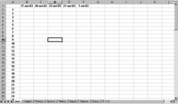
• Now select the entire worksheet, and from the Edit menu choose Copy (usually associated with Ctrl+C shortcut keys). Then position yourself on cell A1 of the second worksheet (“Cagliari”) and click Enter (or from the Edit menu choose Paste – shortcut Ctrl+V). Repeat the Paste operation on all worksheets. Then, in each sheet, position yourself on cell B2 and from the Window menu choose Freeze Panes. This way we can easily scroll rows and columns keeping the first fixed.

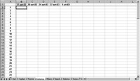
• Now proceed to data entry. Retrieve a complete table of results and delays from the latest draw, perhaps from the Lotto Game website (www.giocodellotto.com) and start entering data for each wheel, i.e., in each sheet. The numbers drawn in that draw will have the delay number “0”. Then verify with the Find command from the Edit menu that there are five “0s” in the draw column. The same operation must be done for all wheels.

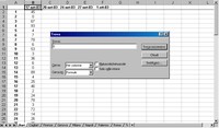
• For the next draw, you can update the delay column semi-automatically by entering the simple formula “=B2+1” in cell C1 on the first sheet. Now drag the cell down the entire column and the delays will be automatically updated. However, it is always necessary to enter “0” manually corresponding to the drawn numbers. To update the other sheets, just copy and paste cell C1 and then drag it down the entire column, always manually entering a “0” for the drawn numbers.

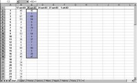
• At the next draw, it will be enough to drag cell C2 to D2 in the first sheet and then drag D2 down the entire D column, or select all relevant cells in column C and drag them to D. In any case, you will have to manually enter “0” for the drawn numbers. The operation must be repeated for all wheels. At the following draw, repeat the procedure moving one column, then selecting the cells in column D and moving them to column E, and so on…

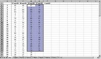
• At this point, we can freely work on our table to check the numbers drawn and the biggest delays. In the worksheet you want to examine, open the Data menu, Filter and choose AutoFilter. Now, to see which numbers came out, for example, in the September 24 draw, go to the corresponding column and click on the AutoFilter arrow. From the drop-down menu select the item 0 and you get the rows of the numbers drawn on that occasion.

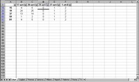
• To return to the full table, click again on the AutoFilter arrow and choose the option (All). Now we are ready for a new analysis. To see the century numbers in the last draw on the Bari wheel, click the AutoFilter arrow in the last draw column and choose Customize. In the dialog box select from the drop-down menu the option is greater than or equal to and enter the value “100”.

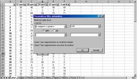
• To create a table of the 10 most delayed numbers for each wheel, in the first sheet click the AutoFilter arrow in the last draw column and choose (Top 10…). Then open the Data menu, Sort. In Sort by, choose the name of the last draw column (“1-Oct-03”) and click Descending. The result is the 10 most delayed numbers on the wheel, ordered from the greatest delay to the least. Repeat the operation on all worksheets.

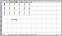
• From the first worksheet open the Insert menu and choose Worksheet. Name this new sheet “Delays Table” with the procedure seen before. Still in the first sheet, now select the cells of the ten delayed numbers, then holding down the Ctrl key also select the delay cells in the last draw column. After the multi-selection, open the Edit menu and choose Copy. Now move to the worksheet of the Delays Table, position yourself in cell B3, then press Enter.

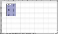
• In the Delays Table sheet select cells B1 and C1, then open the Format menu, Cells. On the Alignment tab choose a Horizontal text alignment “center” and activate the Merge cells box. In the new cell write “Bari”. In cell B2 write “number” and in C2 “delay”. Now select these three cells and drag them to the right to replicate them 4 times, replacing “Bari” with the names of other wheels. Select this result and copy it to B13, changing the wheel names to the missing ones.

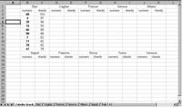
• Now enter the ten most delayed numbers of each wheel by copying and pasting from each worksheet after selecting them with the AutoFilter, as seen before. After finishing data entry, select the cells with the wheel names holding down the Ctrl key. From the Format, Cells menu choose the Font tab and set a Bold style and red color to our text. Then select the entire sheet and choose Format, Cells menu. On the Pattern tab choose white color.

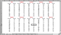
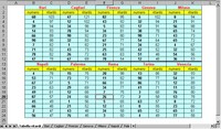
• Now select our data area and from the Format, Cells menu open the Border tab and choose the Default “Box” and “Inside”. From the same menu choose a well-marked line style for the top border of cells with the names of the 5 lower wheels. Then reselect the entire data area and from Format, Cells, Pattern choose a light color. Finally, select all the “number” and “delay” cells holding the Ctrl key and give them a Pattern with a contrasting color. The table is ready for printing.