
All the secrets to building a crossword with Excel, defining the general formatting of the grid and an advanced system for verifying the entered text.

Add us to your preferred sources.

All the secrets to building a crossword with Excel, defining the general formatting of the grid and an advanced system for verifying the entered text.
With this lesson, we present a quick way to create a crossword that is aesthetically pleasing, lightweight, and rich in interactive features, completely innovative compared to what is possible on a paper sheet: dynamic definitions, the possibility of having hints to check errors or correct wrong words.

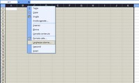
The main characteristic of crosswords is that they consist of a series of square cells inside which letters are written that provide the solutions. In Excel, this structure can be reproduced by first selecting a number of columns and then, after a right-click, defining the same width with the Column Width function..
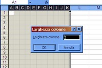
In the window that appears, type the value “2” which makes the width comparable to the default row height, thus creating small squares. At this point, we widen the view to better center the crossword during formatting. We select the columns just formatted plus some to the left and right and choose Selection from the Zoom dropdown menu.
Now we create the borders to delimit the area of our crossword. After selecting all the necessary cells (including two columns to the left left empty for inserting an image), we choose the All Borders formatting from the Borders palette, which is called up from the application menu. Then we frame everything with the Thick Box Border formatting.
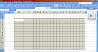
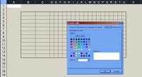
To highlight the drawn structure, we can flatten the sheet, as if it were a printed page. By selecting columns in excess compared to those containing the framed cells, we choose Format > Cells > Pattern and then the white color. Alternatively, you can use the Fill Color palette accessible from the application (bucket icon).
Now we merge the cells that should host the decorative image. We select the cells and after a right-click, we choose Format Cells from the dropdown menu. In the window, we opt for the Alignment tab and then check the Merge Cells box. The result will be a single white space as tall as our crossword.
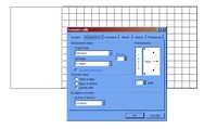
We insert the image. We position ourselves more or less at the height of the empty cell and then choose Insert > Picture > From File.. and browse the PC folders to find a suitable image. Click OK. The inserted file will keep its original dimensions. To modify them, you need to work on its properties directly from Excel, without other graphic-type applications.
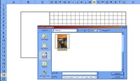
Positioning over the image, with a right-click choose Format Picture from the dropdown menu that appears. Calling up the Size tab, it is possible to set Height and Width by specifying new measurements in cm or proportionally to the original. In the Colors and Lines menu, it is possible to set a border by working on the Line parameter.
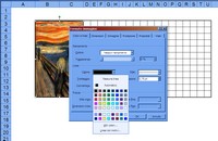
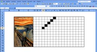
Now we color the black cells. To speed up the process, start by coloring a single cell: select it and with the Fill Color palette of the application (bucket icon) choose black. Select the cell again and choose the Format Painter function (brush icon). A second click on the cell to color and replicate the procedure.
It is now necessary to make all cells behave the same way when entering solutions. Selecting the entire crossword, with a right-click we call up Format Cells. In the window under Alignment > Text Alignment > Horizontal we set Center, and the same for Vertical.
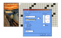
Still in the Format Cells command window, we set the Font type. For Font choose Times New Roman (as in the real Settimana Enigmistica), for Style opt for Regular and 10 for Size. Click OK and we will have the complete crossword structure.
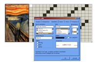
Let’s move on to the definitions. To fully exploit Excel’s potential, we can make each definition appear once the mouse is positioned on the cell that starts a word. To do this, just insert Comments. Let’s do a test: position on the first top-left cell and choose Insert > Comment then write inside the box.
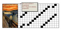
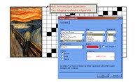
Now right-click on the cell where we just inserted a comment: choose Edit Comment from the menu. Another right-click inside the comment and choose Format Comment: this way, we can change Font type, Color, Size, and Style.
Once all the definitions are inserted, the only thing left is to invent a way to facilitate the filling and checking of answers. For this, you need a copy of the crossword that is invisible to the reader. Select the entire crossword, copy it and paste three rows below the one already created, then insert all the solutions, letter by letter.
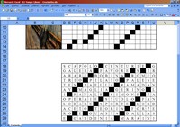
Now we reformat the second crossword with the solutions. We select it and in Format > Cells under the Borders menu choose None, in Pattern select white for Color, while for Font choose white for Color. After OK, every element of the second crossword will disappear by making everything white on white.
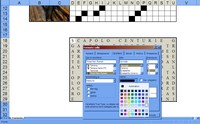
At this point, we insert a trick to provide hints to the person doing the crossword. The mechanism, logically speaking, is simple: every letter written in the main crossword that is wrong is formatted in red. For this, it is necessary to use Excel’s conditional formatting, accessible from Format > Conditional Formatting.
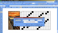
In the window that appears, it is necessary to set all parameters. In the Condition 1 dropdown menu, choose Cell value is.. In the second dropdown menu, choose “not equal to.” At this point, a box automatically appears. Click inside and navigate with the pointer to the corresponding cell in the invisible crossword.
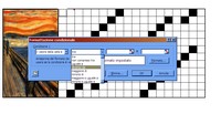
When you select the cell, a value is automatically written. Now, still in the Conditional Formatting window, click Format. In the new window that opens, you will set what to change if the conditions are met. Specifically, we choose to change only Font > Color, selecting red. Then click OK twice.
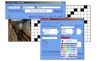
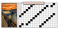
Repeating the operation for the remaining cells, we will have an enhanced multimedia crossword. How does it work? You position yourself on the cells and the definition appears in a comment. Writing the solution, inserting one letter per cell, automatically a red letter will appear if it is wrong, or black if the solution is correct.
Be the first to comment