
Have I already paid the phone bill? When does the electricity bill expire? Questions that at least once we have all asked ourselves. We can keep everything in order thanks to Excel.

Add us to your preferred sources.

Have I already paid the phone bill? When does the electricity bill expire? Questions that at least once we have all asked ourselves. We can keep everything organized thanks to Excel.
First, let’s prepare the worksheet that will contain the overview of our bills. Let’s delete Sheet3 (which is automatically created for every new worksheet) and rename Sheet1 to Bills and Sheet2 to Statistics. In the first sheet, we will enter the received bills, in the second a pivot table that will allow us to observe consumption trends over various periods of the year.

Let’s start with the sheet we named Bills. We need to prepare at least five columns: Bill, Period, Amount, Due Date, Payment. In the first column, we will store the type of bill (e.g., “ENEL”); in the second the reference period (“Jan/Feb 2003”); in the third the amount; in the fourth the due date; and in the fifth the date on which the payment was actually made. Simple, right?
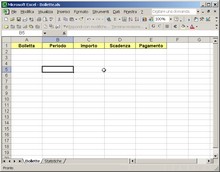
Let’s enter some example data. We can invent them, taking care to choose plausible dates and amounts, or we can dig through a dusty drawer to be sure to have a realistic picture of the situation. Even though this phase is tedious and requires some attention, it immediately allows us to experiment with the more advanced functions of our worksheet and verify that the formulas are correct.

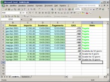
Let’s make things slightly more complicated: now we want Excel to tell us how many days remain until the due date. How can we calculate it? Let’s insert a column called GAS (Days Until Due) and enter in the first cell the formula: =$D2-TODAY() which exactly provides the number of days remaining until the bill’s due date (or a negative number if it has already expired, or zero if it expires today).

Copy the formula down the entire column. This setup is a bit difficult to read because it doesn’t consider the bills that have already been paid. Let’s insert a new column, Status, with the formula =IF($E2<>“”, “Paid”, $E2). Searching for bills is already greatly simplified, but thinking in terms of relative numbers is uncomfortable even for those familiar with algebra. Let’s see how to improve it further.

Let’s modify the third part of the IF statement so that it behaves differently for positive and negative numbers: =IF($E2<>“”, “Paid”, IF($F2<0, "Overdue by " & (-$F2) & " days", "Due in " & $F2 & " days")). It seems complicated, but it allows us first to distinguish between paid and unpaid bills, then between those overdue and those yet to expire. The complexity of the formula is rewarded by the ease of reading.
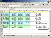
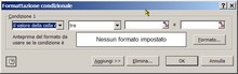
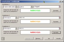
We wonder if we can make our scheme even clearer. Let’s try highlighting texts with conditional formatting. Select the first cell of the Status column, then go to Format/Conditional Formatting menu. The Conditional Formatting dialog box allows you to enter up to three logical conditions and assign different styles to them. This technique highlights particular situations.
Let’s start with the simplest condition: paid bills. Select from the first dropdown “Cell value is”, then “Equal to” from the second, and enter the word “Paid” in the third. Then, by pressing the Format button, choose the style that best fits the case. The style selection is done (almost) exactly as you would from the Format menu. Some options are missing (Number, Alignment, Protection), but we will not need them.
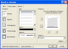
From the Format Cells dialog, you can set borders, background, and font style for cells. In this case, a light green, reassuring and readable, should work. To see the effect of our change, click OK: if the cell contains the word “Paid,” the text color should change. A further step forward in representational clarity. Now let’s deal with the two remaining conditions.

Open the Conditional Formatting window as in point 8. Clicking Add>> insert another condition to handle the case where the bill is not yet overdue. This time we prefer to use a formula to more clearly identify the situation, so select “Formula is” and enter beside it =$F2>=0 and format with orange, perhaps bold, to inspire urgency.
Before closing the window, let’s add another condition based on the formula =$F2
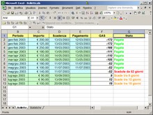
Now in the column, we will have our text appropriately colored depending on the situations, and it will be easy to spot anomalies at a glance. At this point, the GAS column no longer needs to be visible, and we can hide it by right-clicking on the header and choosing Hide. It will continue to be used in formulas but will not take up useful space. To restore it, just use the Unhide command.
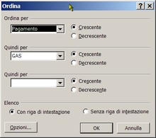
To further improve the functionality of the document, we can use the sort commands from the Data menu. First, select our table (including headers). Then use the Data/Sort command and choose GAS with Descending order. Clicking the OK button, we want our bills with the nearest due dates to be moved to the top of the table.
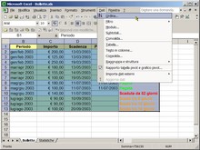
Unfortunately, however, they will be mixed with those already paid. To solve this problem, we use the Sort command again from the Data menu and modify the sorting criteria: first, set Payment/Ascending, second GAS/Ascending. This way, bills already paid will be at the top of the list, and below there will be the others, in order of delinquency. The patience needed to collect the data is rewarded.
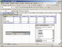
For data analysis, there’s nothing better than a pivot table. Select Data/Pivot Table Report and specify as the source area the table in the Bills sheet and as the destination the Statistics sheet. Then insert the type of bill in the column, the period in the row, and the amount in the center. Using this tool requires some experience, but it provides a range of very interesting perspectives that are easily interchangeable.
Be the first to comment