
If we have taken the big step of going on a diet, we need to keep everything under control: we want to proudly see every lost gram, chart in hand!

Add us to your preferred sources.

If we have taken the big step of going on a diet, we need to keep everything under control: we want to proudly see every lost gram, graph in hand!
Let’s open Excel, click on the File menu and select New… A side panel opens on the right, as shown in the figure, designed to integrate the search for pre-filled templates also on the web. Click on Blank Workbook and immediately save the file with the name controllodieta.xls.

Let’s start entering the dates. When we go on a diet, to avoid becoming paranoid, it is better to set a weekly check frequency. Click on the B to select the entire column (although we will leave the first five rows for summary data that we will enter later) and from the Format menu select Cells.
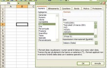
Go to the Number tab, under Category choose Date and in the list select the date display format that seems most convenient. Press Ok and type the first date in cell B7: in our example file it was Sunday 22/05/05. Type the date of the following week, 29/05/05, in the cell below.
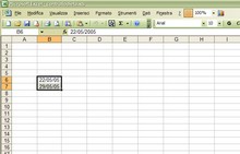
Select both cells and place the cursor over the little square in the bottom right corner of the selection box. As soon as the cursor changes shape, click and drag down and Excel will begin to automatically enter the other dates, with weekly intervals, until you release the mouse button.
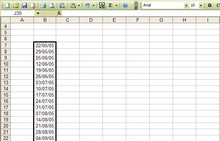
The time interval examined in the example file we are creating, which you can download, is until 31/12/2005. Once the dates are entered, write the labels for the data we will enter. Go to cell C6 and type WEIGHT, CHEST, WAIST, HIPS, BMI, where BMI stands for Body Mass Index.
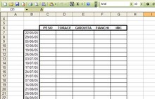
Before starting calculations, let’s finish creating the tables to monitor weight and measurement changes. Continue in row 6, skipping column H, and write Weight Loss, Waist Loss, Hip Loss. To format the text in the cells, from the Format menu select Cells and make the appropriate changes in the Font and Alignment tabs.
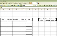
Done, now position yourself in the first cell related to the body mass index and enter the formula =C7/(H*H), where H must be replaced by your height. After that, position the cursor over the little square in the selection box and drag down to copy the formula to the entire column and check the variations in our BMI.

Go to the weight loss control table. Type zero in all three columns in the first row. Position yourself in the second row of the weight loss column table. Here you need to enter a function. It is not enough, in fact, to subtract one series from the next: if the latter has not yet been entered, Excel would return the previous value.
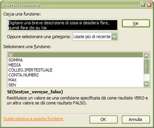
We need to make sure it checks first that the data is different from zero, otherwise it should not perform the operation. Click the Insert Function button in the Formula Bar, in the Dialog Window select IF and press Ok. In the test condition enter C8>0: if true then perform C7-C8, if false then the result should be zero.
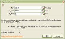
Press Ok in the dialog window and, with the cell still selected, click the little square in the cell selection border and drag down to copy the formula to the entire column. This way we can clearly see how much weight we have lost week by week.
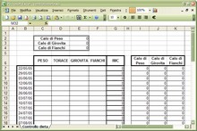
Repeat the same operation regarding the function that calculates the weekly waist measurement loss: create the function with the test condition and then copy it in the column. It will not be necessary to repeat the operation for the third column as, being adjacent to the waist one, it can be copied by dragging from that column.

Return to row two of the document and select cells B and C. Right-click and select Format Cells. In the Alignment tab activate the Merge Cells checkbox. Inside the cell type Weight Loss. Activate the adjacent cell, E2, and activate the AutoSum tool on the Toolbar.
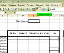
Drag to select the entire range of cells in the Weight Loss column. This way we will have the total pounds lost in the foreground, automatically updated as we enter data in the main table. Repeat the same operation for Waist Loss and Hip Loss.
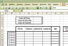
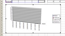
Now select the entire data area, including dates and labels, and from the Insert menu select Chart. Given the type of data, the preferred chart type is area (3D also works). If the table with the values has been correctly selected in the data source section, do not change anything. In the next step customize as preferred and we are done.
Finally, tidy everything up in case we want to print it. First check with the print preview if we can fit the page correctly within the margins (but almost never happens). Then from the View menu activate Page Break Preview and drag the dashed lines to define the print area. And now let’s celebrate the weight loss!

Be the first to comment