
Here’s how to create a series of cards containing the data of the players of your football team in order to check their characteristics, attendance at training sessions, and to be able to compose a true “scientific” lineup.

Add us to your preferred sources.

Here is how to create a series of sheets containing the data of the players of your football team in order to verify their characteristics, attendance frequency at training sessions, and to be able to compile a truly “scientific” lineup.
As the first step, rename Sheet 1 to “Players” by double-clicking on the sheet tab header. Widen column A to enter the full names of all the players. Select twenty rows in column A by clicking with the left mouse button on cell A1 and dragging down to cell A20. Choose bold from the formatting bar (or from the menu Format > Cells, Character tab, Style: bold) and enter the players’ names.

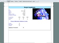
Let’s start creating the players’ personal sheet. Rename Sheet 3 using the name of the player from cell A1 of the Players sheet, in our case Sergio Ingabbiato. Select cells from A1 to H1 and activate the Merge Cells option found under Format > Cells > Alignment tab, and set Horizontal and Vertical alignment to Center. Set the font size to 16 and Style to Bold. Beautify the header with a light blue background pattern.
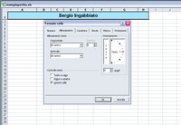
Type the first player’s name in the header cell you just created. Widen column A, select cells from A3 to A18, and in the menu Format > Cells set the text color to dark blue. Enter in the cells the values related to the player’s sheet, in our case Age, Role, Height, Weight, Preferred Foot, Contract Expiry, Championship, appearances, Goals, Monday, Wednesday, and Friday.
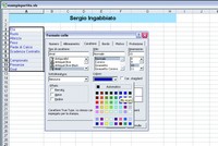
Select and merge (menu Format > Cells, Text Control: Merge Cells) cells from B3-C3 row by row down to B8-C8. From menu Format > Cells, Alignment tab, set Horizontal alignment to right and Vertical alignment to center. Instead set Horizontal and Vertical alignment to center for the text in cells from B10 to D12. Select and merge cells from A14 to D14, then align the text to center horizontally and vertically, and choose the Style (from menu Format > Cells, Character tab) Bold and Font Size 10.
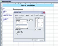
Type “Training Attendance Current Week” in the cells you just modified. Give cells from B16 to B18 the same settings used for cells from B10 to D12. Merge cells A20-B20 and type, after setting Style: Bold from menu Format > Cells, “Add to Lineup”. The cell immediately next to it is particularly important because it will determine the player’s call-up for the match.
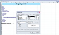
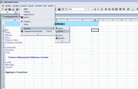
Center-align the text in cell C20 (from menu Format > Cells, Alignment tab) and highlight it using Style: Bold from menu Format > Cells, Character tab. Now insert the player’s picture, obtained previously. Position yourself on cell H2 and open the menu Insert > Image > From file. A dialog window will then open where you can locate the correct path. Then by clicking the Insert button, the photo will appear in the document.
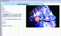
If the image size is not appropriate, use the small squares visible along the image border to drag one of the corners with the mouse until you achieve the desired dimensions. Then move the image using the keyboard arrow keys or by dragging it with the mouse to the top right corner, just below the colored title bar.
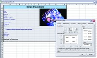
Beautify the sheet by applying a border to the cells (from the formatting bar or from menu Format > Cells, Border tab, Bordered). Now let’s focus on entering all the data related to the player of the sheet just created. Check via a Print Preview from the File menu that all elements fit within the print margins.
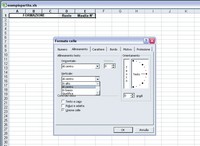
Move to Sheet 2 which we will rename “Lineup”. Merge cells from A1 to C1 row by row down to A16-C16. Select row 1 and center align the text horizontally and vertically and set Style to Bold (from menu Format > Cells, Alignment and Character tabs respectively). Enter “lineup” in the first cell, “Role” in the second, and “Jersey No.” in the third. Now make the automatic filling of the players roster in the lineup.
Now let’s see how to have the names of players that we want to call up by examining the personal sheets (typing “Yes” in the cell corresponding to the entry “add to lineup”) automatically reported in the dedicated sheet. Select A2 and from the menu Insert > Function > Logical use “IF”. Move the cursor to the Test entry and select from the “Sergio Ingabbiato” sheet cell C20 (the one relative to “Yes”) then add =”Yes” to the automatically displayed text string. The resulting string will be:’Sergio Ingabbiato’!C20=”Yes” which will return True.
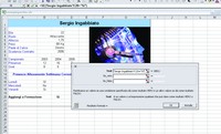
For the If_true entry type the string: MID(‘Sergio Ingabbiato’!A1,1,30) so that if “Yes” is typed in C20 the player’s name will be extracted from the title bar (A1-H1) and displayed in cell A2 of the Lineup sheet. For the If_false entry type a single space so that the application does not display the default False text.
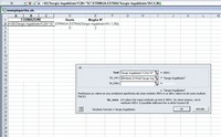
Now do the same combination of actions selecting cell A3 and changing the destination player sheet. Obviously, for the code to work correctly you need to substitute the sheet name in the formula. For example, for the sheet relating to player Giovanni Faccini the full code string will be:
=IF(‘Giovanni Faccini’!C20=”Yes”,MID(‘Giovanni Faccini’!A1,1,30),” “).
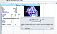
If we want to automatically report the role the player plays, it is possible by selecting the cell related to the role in the Lineup sheet, to use the MID function indicating as Text the cell related to the role in the player sheet (for example ‘Sergio Ingabbiato’!B4), with Start_num=1 and Num_chars=30. The complete string will be: =MID(‘Sergio Ingabbiato’!B4,1,30).
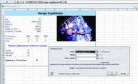
To complete the work, move to the Players sheet. Choosing the players one by one from the menu Insert > Hyperlink > Link To > Insert in Document, select the document part corresponding to the player’s sheet to which the link you are creating must be connected. In the description to display, type “Go to player sheet”.
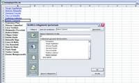
Let’s make a Print Preview from the File menu to ensure that the positions of the elements in the sheets, especially for print margins, are optimal. Adjust spacing between cells to occupy all necessary space to obtain a visually balanced layout. Give greater emphasis to the most interesting texts by using Bold Style, and change the font type according to your taste to make the document more original.
Be the first to comment