
A memorandum created with Excel to keep track of the wedding registry progress, appointments, costs, and details associated with preparing for one of the most important events in life: the wedding.

Add us to your preferred sources.

A memorandum created with Excel to keep track of the wedding gift list progress, appointments, costs, and details associated with preparing one of the most important events in life: the wedding.
This spreadsheet aims to systematize an activity that is usually full of appointments and which, it should not be forgotten, financially exposes a couple: the wedding. After a quick selection of activities, the details will be defined, incorporating each separate task into distinct areas, including columns to define budgets and cells to record important dates not to forget. A summary of this information will help the couple not to get lost between events and costs.

Let’s dive straight into it and create the graphic context within which to insert the tables with the entries related to wedding preparation activities. First of all, let’s build a header for our spreadsheet. Color the cells from A1 to F125 white, just to create a uniform background. Then select the cells, finally, click on the Fill Color icon and choose white. The same must be done, in red, with the cells from A1 to E1.
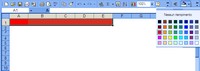
Now merge the previously colored red cells. They must be selected with the mouse, then choose Cells from the Format menu. In the Alignment menu, among the options for Text control, activate both Wrap Text and Merge Cells. Now you can write the title of our sheet inside, taking care to define – again in the Format menu, Cells, but this time Font – a meaningful Font Type and Size (for example, Monotype Corsiva, 36).
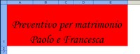
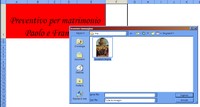
After centering the text (choosing the Center icon related to paragraph formatting) it’s time to add an image. This must already be ready: first select cell F1, then in the Insert menu choose Image, finally From File. A window will appear to browse the PC’s resources. Once the image is found, select it. Then click Insert. In the Excel sheet, the image will be an embedded object, meaning it will be an integral part of the file.
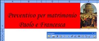
If you click on the inserted image, a palette for modifying its properties will automatically appear. With this, you can increase or decrease the contrast or brightness, crop, rotate, or outline the image with borders, or set a color as transparent. Alternatively, to change the image options, you can right-click and choose Format Picture, which also allows other adjustments.
Let’s now set up the tables below the title. To highlight total costs, create a double line that will contain the most important values of the sheet. To create these lines, select a number of cells equal to the width of the intended area, then click Format Cells, Borders menu. Here choose Custom, the bottom border line, and under Color, open the dropdown and select a color (red). Then repeat the same operation for the next row.
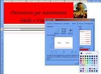
The two red rows created will ultimately include the totals of the expected and actual expenses. After writing in which cells you want to see these amounts displayed, format the cells using a custom method that will automatically place the euro symbol before the figures. This is done by selecting the cells, then Format, Cells, Number. Here choose Currency, leaving two decimal places and the euro symbol in the Symbol option.
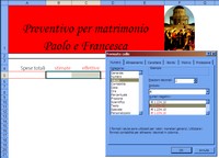
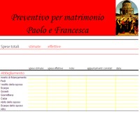
Now let’s move on to the actual tables, which will contain classes of activities or expense contexts. The first concerns “Clothing.” As in step 6, create separation lines that enclose the sequence of topics, then add the entries “Estimated Expenses,” “Actual Expenses,” “Notes,” “Related Appointments,” and “Date.” Enter the expense items, grid them, and color the cell borders using the menu Format, Cells, Borders.
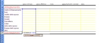
Now the calculation of partial totals is needed for the “Clothing” expenses. Add a new separation line as in step 6. In the first cell write “Total Clothing.” In the cells corresponding to the columns of estimated and actual expenses, add two formulas like “=SUM([Q][x]:[Q][y])”, where [Q] is the column, and [x] and [y] are the starting and ending row of the expense entries. As in point 7, it is advisable to format the content of these cells as Currency.
Besides expenses, there are other issues associated with the listed items. These are appointments and notes. The corresponding cells must be formatted to allow proper data entry. For the cells in the “Appointments” and “Notes” columns, it is necessary to select in Format, Cells, Alignment, the Wrap Text option, while for the cells in the “Date” column, again in Format, Cells, but in the Number menu, you must choose Date.
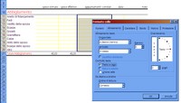
Now, having understood the mechanism used to define a topic, it is necessary to replicate the table formatting operations, insertion of expense entries, and partial expense summation for all other themes. Among the entries we add are “Decorations,” “Gifts,” “Flowers,” “Music,” “Photography,” “Reception,” “Prints,” “Transportation,” and “Miscellaneous,” but each person, according to their idea of a wedding, can remove or add new expense chapters.
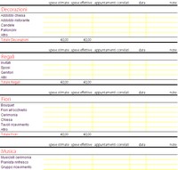
To avoid reformatting the tables from scratch, you can copy and paste the first one, taking care then to change the internal entries. Attention: when pasting, the selected space (measured in cells) must be equal to that of the origin. Once the table is copied, you can add or remove entire rows: after selecting a row, just use the CTRL+ and CTRL- commands. Note well: formulas automatically adjust to the new row numbers.
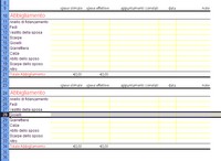
It’s time to tally up. Returning to the top part of the sheet, two formulas must be inserted in the cells where total estimated and actual expenses are to be displayed. Once the cell is selected, enter in the function command line the wording “=SUM(“, followed by the labels of the cells related to the partial totals, separated by a “+”. After entering all addends, close the formula with a parenthesis “)”.

Recommended web pages xnxxyouporn.com, romeoporno.com, xnxxit.com, broporno.org, zzzporno.org, xxx1.link.
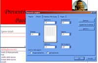
There is nothing left but to print the sheet. However, it is necessary to set up the page: choose Page Setup from the File menu. In the Page menu, select Portrait under Orientation. In the Margins menu, you can save space by lowering the values associated with Header and Footer, since they are empty in our spreadsheet. If you wish, the other margins can also be reduced to gain more printing space.
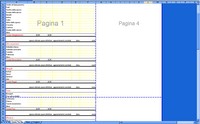
Finally, printing. One last detail, though: the print preview. It is needed to see if the formatted cells fit within the print margins. In the File menu, choose Print Preview. At this point, you can view in the Preview how the page breaks will be divided. To correct any asymmetries or white spaces, you can return to the page margin settings, or edit the spreadsheet to tighten or widen some columns.
Be the first to comment