
A spreadsheet to manage one’s own current account, enter expense items and record credits. Thanks to a clear graphical distinction, it is possible to know whether expenses or savings prevail.

Add us to your preferred sources.

A spreadsheet to manage your own current account, enter expense items and record credits. Thanks to a clear graphic distinction, it is possible to know whether expenses or savings prevail.
This spreadsheet intends to reproduce the typical content of a current account. Since the expense items vary, it is up to the user, once the exercise is finished, to fill in the data according to the statements received from their bank and possibly update the expense categories not foreseen in this sheet. Let’s begin, then. We establish a header with all the data currently useful to define an account, including the European coordinates.

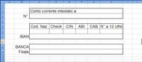
In the first sheet, which we will call “Header” (using the Format menu, Sheet, Rename) we set up three tables as in the image, to host the identifying numbers of an account. The characteristic entries of a current account are: the account holder, the “Account Number”, the “National Code”, the “Check”, the “CIN”, the “ABI”, the “CAB” and the bank details (name and branch). For the IBAN – European coordinate – and the 12-digit account number, we will proceed with the automatic calculation in the next step.
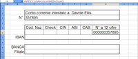
Now enter the account number and calculate the 12-digit identifier. The methods LENGTH ([text]) – which calculates how many characters are in a string [text] – and REPT ([text];[times]) – which writes an alphanumeric value [text] the indicated number of times [times] – are used. This is the formula to calculate the final value: “=REPT(“0″;SUM(12-(LENGTH([accountcell]))))&[accountcell]”. That is, as many zeros are placed before the account number as needed to make 12 digits.
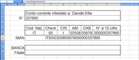
Now we calculate the IBAN. You need to enter all the values in the upper row (“National Code”, “CIN” etc.). To ensure that the values of ABI and CAB keep the zero before the digits (and it is not automatically removed) you need to define the data format with Format, Cells, Number, Text. The IBAN value will be the string resulting from concatenating the indicated values. To join cells just use an “&” as already used in the previous formula. The formula will be of the type: “=[NatCode]&[CIN]&etc.”
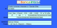
After completing the missing data entry about the reference bank, to make the cover more attractive we add some color. We format the cells with the Borders, Alignment and Pattern menus, in Format, Cells. That is, we add borders, background colors and align the text in the cells consistently. Finally, we insert an image with Insert, Image, From file. The graphic object must already be available on the PC, perhaps downloaded previously from the Internet.
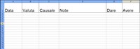
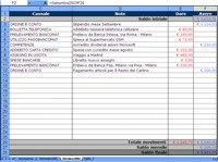
Now let’s move on to the current account. We divide the calculations by months, to make expenses and income more explicit, creating a report at the end. We insert a new sheet, with Insert, Worksheet. Then we rename (with Format, Sheet, Rename) the 3 empty sheets with the names “September2003”, “October2003” and “Balance”. In the first one we set up a table with the entries defining the details of income and expenses: “Date”, “Value Date”, “Reason”, “Notes”, “Debit” and “Credit”.
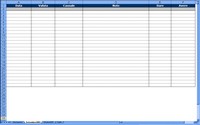
At this point we prepare the table with colors, borders and data types. We select at least 25 rows (the expected transactions for a month), then with Format, Cells, Border we frame everything, using different thicknesses to create separations. Continuing with the same palette, we choose Pattern to color the background. Then with Number we select Date for the columns “Date” and “Value Date”, Text for “Reason” and “Notes”, Currency (also adding the € Symbol) for “Debit” and “Credit”.
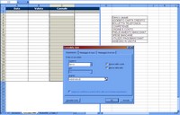
Now we define the reasons to be entered in the current account. The list must be written in a separate table (for example, in column I). After completing it, we select the “Reason” column and choose from the Data menu the Validation option. Under Settings, in the Allow list we opt for List. For the Source entry, instead, we click in the active area, then with the mouse select the cells with the reasons just listed: the range will be entered automatically. Then press OK.
What was established in point 8 allows us to have a pre-filled list to choose from once you click in the cells. So let’s try to enter a series of useful data to simulate some sums in our exercise. To calculate monthly expenses and income we add three final rows (for the “Total of transactions”, the “Monthly balance” and the “Final balance”) and an initial value, corresponding to the “Starting balance”, which for the coming months will be the final balance of the previous month.
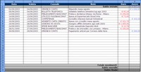
Now let’s move on to the sums. First, we calculate the total expenses. Position yourself in the cell that intersects the “Total of transactions” row with the “Debit” column. Click on the AutoSum icon. The formula using the SUM method and an active area will appear. Use the mouse to take the borders of the area and expand or reduce it to include the cells of the entire expense column. Then press OK and repeat the operation in the next cell, for “Credit”.
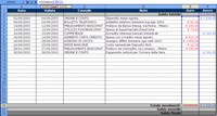
Calculate the monthly balances, placing the result in the cells with blue writing if positive, red if negative. Using the IF method we write the result only if it is consistent with the column that must host it (active or passive), alternatively we report zero. The value is taken as the absolute value (ABS). In the passive cell we use the formula “=IF(([TotCredit]-[TotDebit])<0;ABS([TotCredit]-[TotDebit]);0)". For the active cell, instead, change .
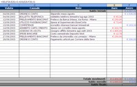
Calculate the final balance placing the result in the right cell, depending on whether it is active or passive. Sum the active balances (initial and monthly) and subtract the passive ones (initial and monthly). If the result is negative, it is written in the passive cell, if positive in the active cell. In the other cell we write zero. The formula is built like the previous one with the IF method, but it has four terms (two positive, two negative). The > and < change in the two cells. The value is taken as absolute (ABS).
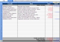
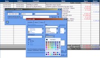
Now let’s make the table more elegant, hiding zeros in the starting, monthly and final balance cells. We use an ad hoc formatting: select, one at a time, the relevant cells, then choose Format and Conditional Formatting. In the appearing window, in Condition 1 put Cell Value Is, then equal to, then type a “0”. Then in Format, change only the Font Color, putting it the same as the cell background, then press OK twice.
Once the table is finished, replicate it in the following months. To speed up you can copy and paste everything done, including the list of reasons. The only precaution is to insert a formula in the starting balance that retrieves the values of the final balance of the previous month. This is the formula: “=[PreviousMonthSheet]![PreviousMonthTotal]”, where [PreviousMonthSheet] is in our case “September2003”, while [PreviousMonthTotal] are E28 and F28 for the passive and active balances.
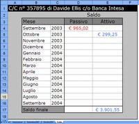
Finally, create a simple table in the “Balance” sheet. Insert the entries “Month”, “Active” and “Passive”. Format the cells like in previous tables, particularly those with monetary values. Finally, report the monthly balance of each month. The method is the same as in step 14. Similarly to step 13, hide zeros. Then at the bottom of the table put a cell for the “Final Balance” where you enter the balance of the last updated month.
Be the first to comment